I/O to and from Gadget2 snapshots

LensTools provides an easy to use API to interact with the Gadget2 binary format (complete documentation in API); you can use the numpy functionality to generate your own position and velocity fields, and then use the LensTools API to write them to a properly formatted Gadget2 snapshot (that you can subsequently evolve with Gadget2). Here’s an example with \(32^3\) particles distributed normally around the center of the box (15 Mpc), with uniform velocities in [-1,1]m/s. First we generate the profiles

>>> from lenstools.simulations import Gadget2SnapshotDE

>>> import numpy as np
>>> from astropy.units import Mpc,m,s

#Generate random positions and velocities
>>> NumPart = 32**3
>>> x = np.random.normal(loc=7.0,scale=5.0,size=(NumPart,3)) * Mpc
>>> v = np.random.uniform(-1,1,size=(NumPart,3)) * m / s

Then we write them to a snapshot

########################Write#################################

#Create an empty gadget snapshot

>>> snap = Gadget2SnapshotDE()

#Put the particles in the snapshot
>>> snap.setPositions(x)
>>> snap.setVelocities(v)

#Generate minimal header
>>> snap.setHeaderInfo()

#Write the snapshot
>>> snap.write("gadget_ic")

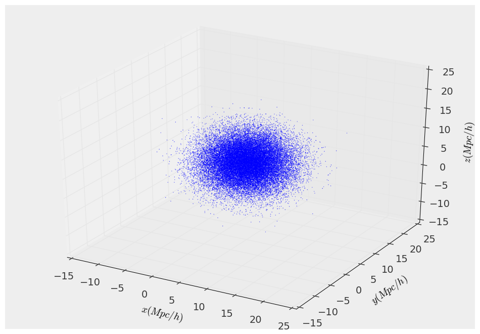
Now check that we did everything correctly, visualizing the snapshot

######################Read and visualize#########################

#Open the snapshot
>>> snap = Gadget2SnapshotDE.open("gadget_ic")

#Visualize the header
>>> print(snap.header)

#Get positions and velocities
>>> snap.getPositions()
>>> snap.getVelocities()

#Visualize the snapshot
>>> snap.visualize(s=1)
>>> snap.savefig("snapshot.png")
>>> snap.close()

This is the result

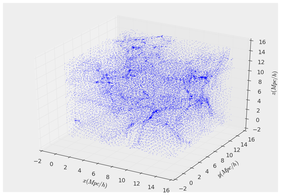
If you don’t believe that this works, here it is what happens with an actual snapshot produced by a run of Gadget2

######################Read and visualize#########################

#Open the snapshot
>>> snap = Gadget2SnapshotDE.open("../Test/Data/gadget/snapshot_001")

#Visualize the header
>>> print(snap.header)

H0 : 72.0 km / (Mpc s)
Ode0 : 0.74
Om0 : 0.26
box_size : 15.0 Mpc/h
endianness : 0
files : ['Test/Data/gadget/snapshot_001']
flag_cooling : 0
flag_feedback : 0
flag_sfr : 0
h : 0.72
masses : [  0.00000000e+00   1.03224800e+10   0.00000000e+00   0.00000000e+00 0.00000000e+00   0.00000000e+00] solMass
num_files : 1
num_particles_file : 32768
num_particles_file_gas : 0
num_particles_file_of_type : [    0 32768     0     0     0     0]
num_particles_file_with_mass : 0
num_particles_total : 32768
num_particles_total_gas : 0
num_particles_total_of_type : [    0 32768     0     0     0     0]
num_particles_total_side : 32
num_particles_total_with_mass : 0
redshift : 2.94758939237
scale_factor : 0.253319152679
w0 : -1.0
wa : 0.0

#Get positions and velocities
snap.getPositions()
snap.getVelocities()

#Visualize the snapshot
snap.visualize(s=1)
snap.savefig("snapshot_gadget.png")

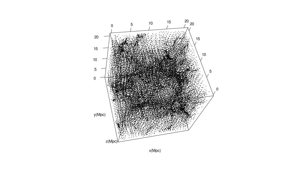
If you wish, you can export the snapshot positions in R format so that you can take full advantage of the RGL graphics library to visualize your snapshot (works a lot better than matplotlib for three dimensional plots):

#Save positions in R format
snap.pos2R("snapshot.rdata",variable_name="pos")

##################################################
#####Then, inside an R console####################
##################################################

library('rgl')
load('snapshot.rdata')
n <- 32^3
plot3d(pos[1:n,1],pos[1:n,2],pos[1:n,3],size=1,xlab='x(Mpc)',ylab='y(Mpc)',zlab='z(Mpc)')
rgl.snapshot( 'snapshot_R.png', fmt = "png", top = TRUE )

which looks something like this

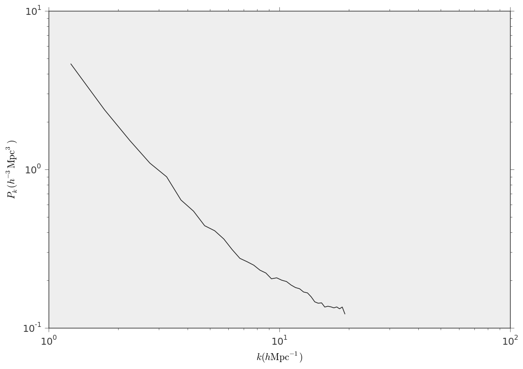
We can also measure the density fluctuations power spectrum \(P_k\), defined as \(\langle \delta n_k \delta n_{k'} \rangle = \delta_D(k+k')P_k\)

#Measure the power spectrum
k_edges = np.arange(1.0,20.0,0.5) * (1/Mpc)
k,Pk = snap.powerSpectrum(k_edges,resolution=64)

#Plot
fig,ax = plt.subplots()

ax.plot(k,Pk)
ax.set_yscale("log")
ax.set_xscale("log")
ax.set_xlabel(r"$k(h\mathrm{Mpc}^{-1})$")
ax.set_ylabel(r"h^{-3}$P_k(\mathrm{Mpc}^3)$")
fig.savefig("snapshot_power_spectrum.png")
snap.close()

Which looks like this