The LensTools Weak Lensing Simulation pipeline
This document is a hands–on tutorial on how to deploy the lenstools weak lensing simulation pipeline on a computer cluster. This will enable you to run your own weak lensing simulations and produce simulated weak lensing fields (shear and convergence) starting from a set of cosmological parameters.
Pipeline workflow
A scheme of the pipeline workflow can be seen in the figure below. The starting point is to select a set of cosmological parameters that are supposed to describe your mock universe (i.e. a combination of \((H_0,\Omega_m,\Omega_b,\Omega_\Lambda,w_0,w_a,\sigma_8,n_s)\)). The first step in the pipeline is running several independent \(N\)–body simulations that will give an accurate picture of the dark matter density field of the universe at different redshifts. Once the \(N\)–body boxes are produced, the multi–lens–plane algorithm is used to trace the deflection of light rays as they go through the simulated density boxes. This will allow to compute background galaxies shape distortions and/or weak lensing quantities such as the shear \(\gamma_{1,2}\) and the convergence \(\kappa\) (and, with a limited accuracy, the rotation angle \(\omega\)).
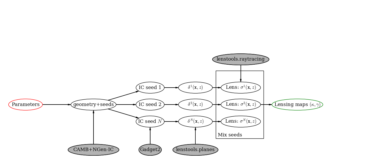
A scheme of the pipeline workflow
In the remainder of the document a detailed scheme of the pipeline is illustrated.
The directory tree
lenstools provides a set of routines for managing the simulations directory tree, which is crucial for organizing the produced files in a sensible way. The first step in the process is creating a new batch of simulations. The way you accomplish this is through a SimulationBatch object.
>>> from lenstools.pipeline.simulation import SimulationBatch
>>> from lenstools.pipeline.settings import EnvironmentSettings
You will need to choose where you want to store your files: in each simulation batch there are two distinct locations files will be saved in. The “home” location is reserved for small files such as code parameter files, tabulated power spectra and other book–keeping necessary files. The “storage” location is used to store large production files, such as \(N\)–body simulation boxes, lensing planes and weak lensing maps. These locations need to be specified upon the batch creation
>>> environment = EnvironmentSettings(home="SimTest/Home",storage="SimTest/Storage")
>>> batch = SimulationBatch(environment)
or, if your settings are contained in a file called environment.ini, you can run the following
>>> batch = SimulationBatch.current("environment.ini")
The contents of environment.ini should look something like
[EnvironmentSettings]

home = SimTest/Home
storage = SimTest/Storage
You will need to specify the home and storage paths only once throughout the execution of the pipeline, lenstools will do the rest! If you want to build a git repository on top of your simulation batch, you will have to install GitPython and initiate the simulation batch as follows
>>> from lenstools.pipeline.remote import LocalGit
>>> batch = SimulationBatch(environment,syshandler=LocalGit())
Cosmological parameters
We first need to specify the cosmological model that will regulate the physics of the universe expansion and evolution of the density perturbations. We do this through the cosmology module of astropy (slightly modified to allow the specifications of parameters like \(n_s\) and \(\sigma_8\)).
>>> from lenstools.pipeline.simulation import LensToolsCosmology
>>> cosmology = LensToolsCosmology(Om0=0.3,Ode0=0.7)
The cosmology object will be initialized with \((\Omega_m,\Omega_\Lambda)=(0.3,0.7)\) and all the other parameters set to their default values
>>> cosmology
LensToolsCosmology(H0=72 km / (Mpc s), Om0=0.3, Ode0=0.7, sigma8=0.8, ns=0.96, w0=-1, wa=0, Tcmb0=2.725 K, Neff=3.04, m_nu=[ 0.  0.  0.] eV, Ob0=0.046)
Now we create a new simulation model that corresponds to the “cosmology” just specified, through our “batch” handler created before
>>> model = batch.newModel(cosmology,parameters=["Om","Ol"])

[+] SimTest/Home/Om0.300_Ol0.700 created on localhost
[+] SimTest/Storage/Om0.300_Ol0.700 created on localhost
The argument “parameters” specifies which cosmological parameters you want to keep track of in your model; this is useful, for example, when you want to simulate different combinations of these parameters while keeping the other fixed to their default values. The values that are specified in the “parameters” list are translated into the names of the attributes of the LensToolsCosmology instance according to the following (customizable) dictionary
>>> batch.environment.name2attr

{'Ob': 'Ob0',
'Ol': 'Ode0',
'Om': 'Om0',
'h': 'h',
'ns': 'ns',
'si': 'sigma8',
'w': 'w0',
'wa': 'wa'}
Note that lenstools informs you of the directories that are created on disk. You have access at any time to the models that are present in your simulation batch
>> batch.models
[<Om=0.300 , Ol=0.700>]
Simulation resolution
It is now time to specify the resolution of the \(N\)–body simulations that will be run to map the 3D density field of the universe. There are two numbers you need to set here, namely size of the box (that will fix the largest mode your simulations will be able to probe) and the number of particles on a side (that will fix the shortest mode). This command will create a collection of simulations with \(512^3\) particles in a box of size 240.0 Mpc/h
>>> collection = model.newCollection(box_size=240.0*model.Mpc_over_h,nside=512)

[+] SimTest/Home/Om0.300_Ol0.700/512b240 created on localhost
[+] SimTest/Storage/Om0.300_Ol0.700/512b240 created on localhost
Again, you will have access at any time to the collections that are present in your model
>>> model = batch.getModel("Om0.300_Ol0.700")
>>> model.collections

[<Om=0.300 , Ol=0.700> | box=240.0 Mpc/h,nside=512]
Initial conditions
Each simulation collection can have multiple realizations of the density field; these realizations share all the same statistical properties (i.e. the matter power spectrum), but have different spatial arrangements of the particles. This allows you to measure ensemble statistics such as means and covariances of various observables. Let’s add three independent realizations of the density field to the “512b240” collection, with random seeds 1,22,333 (the random seed will be used by the initial condition generator to produce different density fields that share the same 3D power spectum)
>>> for s in [1,22,333]:
        collection.newRealization(seed=s)

[+] SimTest/Home/Om0.300_Ol0.700/ic1 created on localhost
[+] SimTest/Storage/Om0.300_Ol0.700/ic1 created on localhost
[+] SimTest/Home/Om0.300_Ol0.700/ic2 created on localhost
[+] SimTest/Storage/Om0.300_Ol0.700/ic2 created on localhost
[+] SimTest/Home/Om0.300_Ol0.700/ic3 created on localhost
[+] SimTest/Storage/Om0.300_Ol0.700/ic3 created on localhost
At this point it should not be surprising that you can do this
>>> collection.realizations

[<Om=0.300 , Ol=0.700> | box=240.0 Mpc/h,nside=512 | ic=1,seed=1 | IC files on disk: 0 | Snapshot files on disk: 0,
<Om=0.300 , Ol=0.700> | box=240.0 Mpc/h,nside=512 | ic=2,seed=22 | IC files on disk: 0 | Snapshot files on disk: 0,
<Om=0.300 , Ol=0.700> | box=240.0 Mpc/h,nside=512 | ic=3,seed=333 | IC files on disk: 0 | Snapshot files on disk: 0]
Note that, at this step, we are only laying down the directory tree of the simulation batch, and you can see that there are neither IC files nor snapshot files saved on disk yet (this will be produced when we actually run the simulations, but this will be explained later in the tutorial).
Lens planes
For each of the realizations in the collection, we have to create a set of lens planes, that will be necessary for the execution of the ray–tracing step via the multi–lens–plane algorithm. The settings for these lens plane set can be specified through a INI configuration file. Let’s call this file “planes.ini”; it should have the following structure
[PlaneSettings]

directory_name = Planes
override_with_local = False
format = fits
plane_resolution = 128
first_snapshot = 0
last_snapshot = 58
cut_points = 10.71
thickness = 3.57
length_unit = Mpc
normals = 0,1,2

#Customizable, but optional
name_format = snap{0}_{1}Plane{2}_normal{3}.{4}
snapshots = None
kind = potential
smooth = 1
Once you specified the plane configuration file, you can go ahead and create a lens plane set for each of the \(N\)–body realizations you created at the previous step
>>> from lenstools.pipeline.settings import PlaneSettings
>>> plane_settings = PlaneSettings.read("planes.ini")
>>> for r in collection.realizations:
        r.newPlaneSet(plane_settings)

[+] SimTest/Home/Om0.300_Ol0.700/ic1/Planes created on localhost
[+] SimTest/Storage/Om0.300_Ol0.700/ic1/Planes created on localhost
[+] SimTest/Home/Om0.300_Ol0.700/ic2/Planes created on localhost
[+] SimTest/Storage/Om0.300_Ol0.700/ic2/Planes created on localhost
[+] SimTest/Home/Om0.300_Ol0.700/ic3/Planes created on localhost
[+] SimTest/Storage/Om0.300_Ol0.700/ic3/Planes created on localhost
To summarize what you just did, as usual you can type
>>> for r in collection.realizations:
        r.planesets

[<Om=0.300 , Ol=0.700>  |  box=240.0 Mpc/h,nside=512  |  ic=1,seed=1  | Plane set: Planes , Plane files on disk: 0]
[<Om=0.300 , Ol=0.700>  |  box=240.0 Mpc/h,nside=512  |  ic=2,seed=22  | Plane set: Planes , Plane files on disk: 0]
[<Om=0.300 , Ol=0.700>  |  box=240.0 Mpc/h,nside=512  |  ic=3,seed=333  | Plane set: Planes , Plane files on disk: 0]
Weak lensing fields
The last step in the pipeline is to run the multi–lens–plane algorithm through the sets of lens planes just created. This will compute all the ray deflections at each lens crossing and derive the corresponding weak lensing quantities. The ray tracing settings need to be specified in a INI configuration file, that for example we can call “lens.ini”. The following configuration will allow you to create square weak lensing simulated maps assuming all the background sources have the same redshift
[MapSettings]

directory_name = Maps
override_with_local = False
format = fits
map_resolution = 128
map_angle = 3.5
angle_unit = deg
source_redshift = 2.0

#Random seed used to generate multiple map realizations
seed = 0

#Set of lens planes to be used during ray tracing
plane_set = Planes

#N-body simulation realizations that need to be mixed
mix_nbody_realizations = 1,2,3
mix_cut_points = 0,1,2
mix_normals = 0,1,2
lens_map_realizations = 4

#Which lensing quantities do we need?
convergence = True
shear = True
omega = True

#Customizable, but optional
plane_format = fits
plane_name_format = snap{0}_potentialPlane{1}_normal{2}.{3}
first_realization = 1
Different random realizations of the same weak lensing field can be obtained drawing different combinations of the lens planes from different \(N\)–body realizations (mix_nbody_realizations), different regions of the \(N\)–body boxes (mix_cut_points) and different rotation of the boxes (mix_normals). We create the directories for the weak lensing map set as usual
>>> from lenstools.pipeline.settings import MapSettings
>>> map_settings = MapSettings.read("lens.ini")
>>> map_set = collection.newMapSet(map_settings)

[+] SimTest/Home/Om0.300_Ol0.700/Maps created on localhost
[+] SimTest/Storage/Om0.300_Ol0.700/Maps created on localhost
And, of course, you can check what you just did
>>> collection.mapsets

[<Om=0.300 , Ol=0.700> | box=240.0 Mpc/h,nside=512 | Map set: Maps | Map files on disk: 0 ]
Now that we layed down our directory tree in a logical and organized fashion, we can proceed with the deployment of the simulation codes. The outputs of these codes will be saved in the “storage” portion of the simulation batch.
Pipeline deployment
After the creation of the directory tree that will host the simulation products (which you can always update calling the appropriate functions on your SimulationBatch instance), it is time to start the production running the actual simulation codes. This implementation of the lensing pipeline relies on three publicly available codes (CAMB , NGenIC and Gadget2) which you have to obtain on your own as the lenstools authors do not own publication rights on them. On the other hand, the lens plane generation and ray–tracing algorithms are part of the lenstools suite. In the remainder of the tutorial, we show how to deploy each step of the pipeline on a computer cluster.
Matter power spectra (CAMB)
The Einstein-Boltzmann code CAMB is used at the first step of the pipeline to compute the matter power spectra that are necessary to produce the initial conditions for the \(N\)–body runs. CAMB needs its own parameter file to run, but in order to make things simpler, lenstools provides the CAMBSettings class. Typing
>>> import lenstools
>>> from lenstools.pipeline.settings import CAMBSettings
>>> camb_settings = CAMBSettings()
You will have access to the default settings of the CAMB code; you can edit these settings to fit your needs, and then generate the INI parameter file that CAMB will need to run
>>> environment = EnvironmentSettings(home="SimTest/Home",storage="SimTest/Storage")
>>> batch = SimulationBatch(environment)
>>> collection = batch.models[0].collections[0]
>>> collection.writeCAMB(z=0.0,settings=camb_settings)

[+] SimTest/Home/Om0.300_Ol0.700/512b240/camb.param written on localhost
This will generate a CAMB parameter file that can be used to compute the linear matter power spectrum at redshift \(z=0.0\) (which NGenIC will later scale to the initial redshift of your \(N\)–body simulation). You will now need to run the CAMB executable to compute the matter power spectrum as specified by the settings you chose. For how to run CAMB on your computer cluster please refer to the jobs section. The basic command you have to run to generate the job submission scripts is, in a shell
lenstools.submission -e SimTest/Home/environment.ini -j job.ini -t camb SimTest/Home/collections.txt
Initial conditions (NGenIC)
After CAMB finished running, it is time to use the computed matter power spectra to generate the particle displacement field (corresponding to those power spectra) with NGenIC. The NGenIC code needs its own parameter file to run, which can be quite a hassle to write down yourself. Luckily lenstools provides the NGenICSettings class to make things easy:
>>> from lenstools.pipeline.settings import NGenICSettings
>>> ngenic_settings = NGenICSettings()
>>> ngenic_settings.GlassFile = lenstools.data("dummy_glass_little_endian.dat")
You can modify the attributes of the ngenic_settings object to change the settings to your own needs. There is an additional complication: NGenIC needs the tabulated matter power spectra in a slightly different format than CAMB outputs. Before generating the NGenIC parameter file we will need to make this format connversion
>>> collection.camb2ngenic(z=0.0)
[+] CAMB matter power spectrum at SimTest/Home/Om0.300_Ol0.700/512b240/camb_matterpower_z0.000000.txt converted into N-GenIC readable format at SimTest/Home/Om0.300_Ol0.700/512b240/ngenic_matterpower_z0.000000.txt
Next we can generate the NGenIC parameter file
>>> for r in collection.realizations:
        r.writeNGenIC(ngenic_settings)

[+] NGenIC parameter file SimTest/Home/Om0.300_Ol0.700/512b240/ic1/ngenic.param written on localhost
[+] NGenIC parameter file SimTest/Home/Om0.300_Ol0.700/512b240/ic2/ngenic.param written on localhost
[+] NGenIC parameter file SimTest/Home/Om0.300_Ol0.700/512b240/ic3/ngenic.param written on localhost
For directions on how to run NGenIC on a computer cluster you can refer to the jobs section. After the initial conditions files have been produced, you can check that they are indeed present on the storage portion of the directory tree
>>> for r in collection.realizations:
        print(r)

<Om=0.300 , Ol=0.700> | box=240.0 Mpc/h,nside=512 | ic=1,seed=1 | IC files on disk: 256 | Snapshot files on disk: 0
<Om=0.300 , Ol=0.700> | box=240.0 Mpc/h,nside=512 | ic=2,seed=22 | IC files on disk: 256 | Snapshot files on disk: 0
<Om=0.300 , Ol=0.700> | box=240.0 Mpc/h,nside=512 | ic=3,seed=333 | IC files on disk: 256 | Snapshot files on disk: 0
Note that the IC file count increased from 0 to 256, but the snapshot count is still 0 (because we didn’t run Gadget yet). We will explain how to run Gadget2 in the next section. The basic command you have to run to generate the job submission scripts is, in a shell
lenstools.submission -e SimTest/Home/environment.ini -j job.ini -t ngenic SimTest/Home/realizations.txt
Gravitational evolution (Gadget2)
The next step in the pipeline is to run Gadget2 to evolve the initial conditions in time. Again, the Gadget2 tunable settings are handled by lenstools via the Gadget2Settings:
>>> from lenstools.pipeline.settings import Gadget2Settings
>>> gadget_settings = Gadget2Settings()
In the gadget_settings instance, you may want to be especially careful in selecting the appropriate values for the OutputScaleFactor and NumFilesPerSnapshot attributes, which will direct which snapshots will be written to disk and in how many files each snapshot will be split. You can generate the Gadget2 parameter file just typing
>>> for r in collection.realizations:
        r.writeGadget2(gadget_settings)

[+] Gadget2 parameter file SimTest/Home/Om0.300_Ol0.700/512b240/ic1/gadget2.param written on localhost
[+] Gadget2 parameter file SimTest/Home/Om0.300_Ol0.700/512b240/ic2/gadget2.param written on localhost
[+] Gadget2 parameter file SimTest/Home/Om0.300_Ol0.700/512b240/ic3/gadget2.param written on localhost
Now you can submit the Gadget2 runs following the directions in the jobs section. The basic command you have to run to generate the job submission scripts is, in a shell
lenstools.submission -e SimTest/Home/environment.ini -j job.ini -t gadget2 SimTest/Home/realizations.txt
If Gadget2 ran succesfully and produced the required snapshot, this should reflect on your SimulationIC instances
>>> for r in collection.realizations:
        print(r)

<Om=0.300 , Ol=0.700> | box=240.0 Mpc/h,nside=512 | ic=1,seed=1 | IC files on disk: 256 | Snapshot files on disk: 976
<Om=0.300 , Ol=0.700> | box=240.0 Mpc/h,nside=512 | ic=2,seed=22 | IC files on disk: 256 | Snapshot files on disk: 976
<Om=0.300 , Ol=0.700> | box=240.0 Mpc/h,nside=512 | ic=3,seed=333 | IC files on disk: 256 | Snapshot files on disk: 976
You have access to each of the \(N\)–body simulation snapshots through the Gadget2Snapshot class.
Lens planes
Now that Gadget2 has finished the execution, we are ready to proceed in the next step in the pipeline. The multi–lens–plane algorithm approximates the matter distribution between the observer and the backround source as a sequence of parallel lens planes with a local surface density proportional to the density constrast measured from the 3D \(N\)–body snapshots. lenstools provides an implementation of the density and lensing potential estimation algorithms. You will have to use the same INI configuration file used to create the planes section of the directory tree (in the former we called this file “planes.ini”). After filling the appropriate section of “job.ini” as outlined in jobs (using “lenstools.planes-mpi” as the executable name), run on the command line
lenstools.submission -e SimTest/Home/environment.ini -o planes.ini -j job.ini -t planes SimTest/Home/realizations.txt
This will produce the plane generation execution script that, when executed, will submit your job on the queue. If lenstools.planes-mpi runs correctly, you should notice the presence of the new plane files
>>> for r in collection.realizations:
        print(r.planesets[0])

<Om=0.300 , Ol=0.700>  |  box=15.0 Mpc/h,nside=32  |  ic=1,seed=1  | Plane set: Planes , Plane files on disk: 178
<Om=0.300 , Ol=0.700>  |  box=15.0 Mpc/h,nside=32  |  ic=2,seed=22  | Plane set: Planes , Plane files on disk: 178
<Om=0.300 , Ol=0.700>  |  box=15.0 Mpc/h,nside=32  |  ic=3,seed=333  | Plane set: Planes , Plane files on disk: 178
You can access each plane through the PotentialPlane class.
Weak lensing fields \(\gamma,\kappa,\omega\)
Once the lensing potential planes have been created, we are ready for the last step in the pipeline, namely the multi–lens–plane algorithm execution which will produce the simulated weak lensing fields. You will need to use the configuration file “lens.ini” that you used to create the maps section of the directory tree in the weak lensing fields section. Here is the relevant extract of the file
[MapSettings]

directory_name = Maps
override_with_local = True
format = fits
map_resolution = 128
map_angle = 3.5
angle_unit = deg
source_redshift = 2.0

#Random seed used to generate multiple map realizations
seed = 0

#Set of lens planes to be used during ray tracing
plane_set = Planes

#N-body simulation realizations that need to be mixed
mix_nbody_realizations = 1,2,3
mix_cut_points = 0,1,2
mix_normals = 0,1,2
lens_map_realizations = 4

#Which lensing quantities do we need?
convergence = True
shear = True
omega = True
Note the change “override_with_local=False”, which became “override_with_local=True”; this is an optional simplification that you can take advantage of if you want. If this switch is set to true, the ray–tracing script will ignore everyting below the “override_with_local” line and read the remaining options from the “Maps” directory. This is a failsafe that guarantees that the weak lensing fields will be generated using the settings that were originally intended for them, i.e. the ones that you used to create the “Maps” directory in the tree.
After filling the appropriate section of “job.ini” as outlined in jobs (using “lenstools.raytracing-mpi” as the executable name), run on the command line
lenstools.submission -e SimTest/Home/environment.ini -o lens.ini -j job.ini -t raytracing SimTest/Home/collections.txt
Where “collections.txt”, in this case, should be a text file with only one line
Om0.300_Ol0.700|512b240
After lenstools.raytracing-mpi finished the execution, you will find your weak lensing maps in the “Maps” directory, and you can conveniently access them through the ConvergenceMap and ShearMap classes.
>>> from lenstools import ConvergenceMap
>>> collection.mapsets

[<Om=0.300 , Ol=0.700> | box=15.0 Mpc/h,nside=32 | Map set: Maps | Map files on disk: 12 ]

>>> mp = collection.mapsets[0]
>>> mp.path("WLconv_z2.00_0001r.fits")

"SimTest/Storage/Om0.300_Ol0.700/32b15/Maps/WLconv_z2.00_0001r.fits"

>>> c = ConvergenceMap.load(mp.path("WLconv_z2.00_0001r.fits"))
>>> c.info

Pixels on a side: 128
Pixel size: 98.4375 arcsec
Total angular size: 3.5 deg
lmin=1.0e+02 ; lmax=9.3e+03
If you need to generate the weak lensing simulated fields not in image form but in catalog form, you can use the SimulationCatalog class instead of the SimulationMaps class
>>> lenstools.showData("catalog_default.ini")

[CatalogSettings]

#Name of catalog batch
directory_name = Catalog
input_files = galaxy_positions.fits
total_num_galaxies = 1000
catalog_angle_unit = deg

#Use the options generated at the moment of the batch generation (advised)
override_with_local = True

#Format of the simulated catalog files
format = fits

#Random seed used to generate multiple catalog realizations
seed = 0

#Set of lens planes to be used during ray tracing
plane_set = Planes

#N-body simulation realizations that need to be mixed
mix_nbody_realizations = 1
mix_cut_points = 0
mix_normals = 0
lens_catalog_realizations = 1

>>> from lenstools.pipeline.settings import CatalogSettings
>>> catalog_settings = CatalogSettings.read(lenstools.data("catalog_default.ini"))
>>> collection.newCatalog(catalog_settings)

[+] SimTest/Home/Om0.300_Ol0.700/Catalog created on localhost
[+] SimTest/Storage/Om0.300_Ol0.700/Catalog created on localhost
Computer cluster offload
Generating job submission scripts
Each computer cluster comes with its own computing environment, its own job scheduler and its own job scheduler directives. To accomodate these differences, lenstools provides a platform–independent interface to generate your submission scripts. The job settings are read from a platform–independent INI configuration file, which is passed to a JobHandler instance. This job handler instance will translate the user provided settings into the machine specific job directives. This provides a platform–independent job deployment. Here is an example of the job submission options for a Gadget2 run, which we will call “job.ini”
[Gadget2]

#Personal settings
email = apetri@phys.columbia.edu
charge_account = TG-AST140041

#Path to executable
path_to_executable = /my/cluster/path/to/the/Gadget2/executable

#Name of the job, output
job_name = Gadget2
redirect_stdout = gadget.out
redirect_stderr = gadget.err

#Resources
cores_per_simulation = 256
queue = development
wallclock_time = 02:00:00

#Script name
job_script_file = gadget.sh
lenstools provides a command line script, lenstools.submission, that will take care of the script generation. The “-s” flag can be used to specify the system we are running on; if not specified, the system is detected automatically looking at the value of the “THIS” environment variable. For example the “-s Stampede” option will generate the submission scripts for the Stampede computer cluster through the StampedeHandler job handler. Here it is an example on how the script is generated: from the command line run
lenstools.submission -e SimTest/Home/environment.ini -j job.ini -t gadget2 -s Stampede SimTest/Home/realizations.txt
or, if you prefer, lenstools.submission can read from stdin too, and hence you can use shell pipes
cat SimTest/Home/realizations.txt | lenstools.submission -e SimTest/Home/environment.ini -j job.ini -t gadget2 -s Stampede
In short, the “-e” switch will make sure that we are pointing to the right simulation batch, the “-j” switch will point to the correct platform–independent job option file, the “-t” switch specifies which job submission script we are generating and the realizations.txt file contains a list of the realizations that the script will process. For example if the contents of “realizations.txt” are
Om0.300_Ol0.700|512b240|ic1
Om0.300_Ol0.700|512b240|ic2
Om0.300_Ol0.700|512b240|ic3
the job submission will process the Om0.300_Ol0.700 model, collection of simulations with \(512^3\) particles and 240.0Mpc/h box size, initial conditions from 1 to 3. You can additionally specify the –chunks and –one options to change the number of simulations that are processed in parallel.
lenstools.submission -e SimTest/Home/environment.ini -j job.ini -t gadget2 -s Stampede SimTest/Home/realizations.txt --chunks 3
will generate 3 job submission scripts, each of which will take care of one of the initial conditions
lenstools.submission -e SimTest/Home/environment.ini -j job.ini -t gadget2 -s Stampede SimTest/Home/realizations.txt --chunks 3 --one
will generate one job submission script, in which the 3 initial conditions are processed one after the other, starting with the first. This job will run on 256 cores
lenstools.submission -e SimTest/Home/environment.ini -j job.ini -t gadget2 -s Stampede SimTest/Home/realizations.txt
will generate one submission script, in which the 3 initial conditions are processed in parallel. This job will run on 768 cores. This is the output of this execution of lenstools.submission
[*] Environment settings for current batch read from SimTest/Home/environment.ini
[+] Using job handler for system Stampede
[*] Current batch home directory: SimTest/Home
[*] Current batch mass storage: SimTest/Storage
[*] Realizations to include in this submission will be read from realizations.txt
[+] Found 3 realizations to include in job submission, to be split in 1 chunks
[+] Generating Gadget2 submission script
[*] Reading job specifications from jobs.ini section Gadget2
[+] Stdout will be directed to SimTest/Home/Logs/gadget.out
[+] Stderr will be directed to SimTest/Home/Logs/gadget.err
[+] SimTest/Home/Jobs/gadget1.sh written on localhost
On Stampede you submit the jobs to the queue using the “sbatch” command:
sbatch SimTest/Home/Jobs/gadget1.sh
Generic job submissions
lenstools provides functionality to distribute execution of arbitrary code throughout all your simulation batch. Suppose that you compiled an executable “myexec” for your own purposes; if this executable accepts the “-e” and “-c” options, i.e. you can run it like this
mpiexec -n 16 ./myexec -e SimTest/Home/environment.ini -c code_options.ini "Om0.300_0.700|512b240|ic1"
Then lenstools.submission can help you distribute the myexec execution across your simulation batch: you just have to include the following section in your “job.ini”
[/path/to/myexec]

#Personal settings
email = apetri@phys.columbia.edu
charge_account = TG-AST140041

#Name of the job, output
job_name = myexecJob
redirect_stdout = myexec.out
redirect_stderr = myexec.err

#Resources
cores_per_simulation = 16
queue = development
wallclock_time = 02:00:00

#Script name
job_script_file = myexec.sh
And, in a shell, type
lenstools.submission -e SimTest/Home/environment.ini -o code_options.ini -j job.ini -t "/path/to/myexec" SimTest/Home/realizations.txt
to generate the submission script.
Job handlers for different clusters
Each computer cluster comes with its own job sheduler and job submission directives. lenstools facilitates the transition between clusters by translating the platform–independent options contained in “job.ini” into cluster specific directives through the JobHandler objects. Currently the “-s” switch that you can pass to lenstools.submission accepts the values “Stampede” (that will select the StampedeHandler handler) and “edison” (that will select EdisonHandler). Should you want to use a different computer cluster, this is what you have to do. Create a file called mycluster.ini, and fill it according to this template (changing the values of the options to adapt to your own cluster)
[Directives]

directive_prefix = #SBATCH
job_name_switch = -J
stdout_switch = -o
stderr_switch = -e
num_cores_switch = -n
num_nodes_switch = -N
tasks_per_node_switch = None
queue_type_switch = -p
wallclock_time_switch = -t
user_email_switch = --mail-user=
user_email_type = --mail-type=all

[ClusterSpecs]

shell_prefix = #!/bin/bash
execution_preamble = None
charge_account_switch = -A
job_starter = ibrun
cores_per_node = 16
memory_per_node = 32
memory_unit = Gbyte
cores_at_execution_switch = -n
offset_switch = -o
wait_switch = wait
multiple_executables_on_node = True
After doing this, you just need to pass the cluster configuration file name “mycluster.ini” to the “-s” switch when you run lenstools.submission and you are all set!
Post processing
This section shows an example on how to do some post processing on the products of your simulation batch (for example measuring the \(N\)–body simulations power spectra). The basic idea is to define a function with the signature
>>> def methodThatMeasuresSomething(pool,batch,settings,node_id,**kwargs):
        ...
where
- pool is a
MPIWhirlPoolinstance that will take care of the parallelization of the code - batch is the simulation batch object, i.e. an instance of
SimulationBatch - settings are the tunable settings of the code
- node_id is the particular batch subset to process, for example “Om0.300_Ol0.700|512b240|ic1”
- kwargs are any other keyword arguments you may want to pass to the methodThatMeasuresSomething method
lenstools will take care of distributing the methodThatMeasuresSomething calls on the computer cluster you are running on. Below is a working example of how to measure the 3D matter power spectrum out of the simulation boxes.
Example: measure the 3D matter power spectrum
Create a file “matter_power_spectrum.py”
###################################################################################
################Measure statistics out of N-body simulation snapshots##############
###################################################################################

import sys,os
import logging

from distutils import config
from ConfigParser import NoOptionError

from lenstools.utils import MPIWhirlPool

from lenstools.simulations.nbody import NbodySnapshot
from lenstools.simulations.gadget2 import Gadget2SnapshotDE
from lenstools.simulations.logs import logdriver

from lenstools.pipeline.simulation import SimulationBatch

import numpy as np
import astropy.units as u

#Orchestra director of the execution
def powerSpectrumExecution():

        script_to_execute = matterPowerSpectrum
        settings_handler = PowerSpectrumSettings
        kwargs = {"fmt":Gadget2SnapshotDE}

        return script_to_execute,settings_handler,kwargs

################################################################
################Snapshot power spectrum#########################
################################################################

def matterPowerSpectrum(pool,batch,settings,node_id,**kwargs):

        assert "fmt" in kwargs.keys()
        fmt = kwargs["fmt"]

        #Safety type check
        assert isinstance(pool,MPIWhirlPool) or (pool is None)
        assert isinstance(batch,SimulationBatch)
        assert isinstance(fmt(),NbodySnapshot)
        assert isinstance(settings,PowerSpectrumSettings)

        #Split the id into the model,collection and realization parts
        cosmo_id,geometry_id = node_id.split("|")

        #Get a handle on the simulation model
        model = batch.getModel(cosmo_id)

        #Scale the box size to the correct units
        nside,box_size = geometry_id.split("b")
        box_size = float(box_size)*model.Mpc_over_h

        #Get the handle on the collection
        collection = model.getCollection(box_size,nside)

        #Log the power spectrum settings to the user
        if (pool is None) or (pool.is_master()):

                logdriver.info("Measuring power spectrum for Ensemble {0}".format(settings.ensemble_name))
                logdriver.info("The Ensemble will be built with the following N-body realizations: {0}".format("-".join([ str(n) for n in settings.nbody_realizations ])))
                logdriver.info("First snapshot: {0}".format(settings.first_snapshot))
                logdriver.info("Last snapshot: {0}".format(settings.last_snapshot))
                logdriver.info("Minimum wavenumber: {0}".format(settings.kmin.to(model.Mpc_over_h**-1)))
                logdriver.info("Maximum wavenumber: {0}".format(settings.kmax.to(model.Mpc_over_h**-1)))
                logdriver.info("Bin size: {0}".format(((settings.kmax-settings.kmin)/settings.num_k_bins).to(model.Mpc_over_h**-1)))
                logdriver.info("FFT grid size: {0}".format(settings.fft_grid_size))
                logdriver.info("Number of bins: {0}".format(settings.num_k_bins))

                #Create dedicated ensemble directory
                ensemble_dir = os.path.join(collection.home_subdir,settings.ensemble_name)
                if not os.path.isdir(ensemble_dir):
                        os.mkdir(ensemble_dir)

        #Construct the array of bin edges
        k_egdes  = np.linspace(settings.kmin,settings.kmax,settings.num_k_bins+1).to(model.Mpc_over_h**-1)

        #Placeholder for the density MPI communications
        density_placeholder = np.empty((settings.fft_grid_size,)*3,dtype=np.float32)
        if pool is not None:
                pool.openWindow(density_placeholder)

                if pool.is_master():
                        logdriver.debug("Opened density window of type {0}".format(pool._window_type))

        #Cycle over snapshots
        for n in range(settings.first_snapshot,settings.last_snapshot+1):

                #Allocate memory for the power spectrum ensemble
                power_ensemble = np.zeros((len(settings.nbody_realizations),settings.num_k_bins)) * (model.Mpc_over_h**3)

                #Log to user
                if (pool is None) or (pool.is_master()):
                        logdriver.info("Processing snapshot {0} of model {1}".format(n,node_id))
                        logdriver.info("Allocated memory for power spectrum Ensemble {0}".format(power_ensemble.shape))

                for r,ic in enumerate(settings.nbody_realizations):

                        #Log to user
                        if (pool is None) or (pool.is_master()):
                                logdriver.info("Processing N-body realization {0}".format(ic))

                        #Instantiate the appropriate SimulationIC object
                        realization = collection.getRealization(ic)

                        #Open the snapshot, measure the power spectrum and close it
                        if pool is not None:
                                if realization.gadget_settings.NumFilesPerSnapshot!=pool.size+1:
                                        logdriver.error("The number of snapshots written in parallel {0} does not coincide with the number of MPI processes {1}!".format(realization.gadget_settings.NumFilesPerSnapshot,pool.size+1))
                                        sys.exit(1)

                        snap = fmt.open(realization.snapshotPath(n,sub=None),pool=pool)
                        k,power_ensemble[r],hits = snap.powerSpectrum(k_egdes,resolution=settings.fft_grid_size,return_num_modes=True,density_placeholder=density_placeholder)
                        snap.close()

                        #Safety barrier sync
                        if pool is not None:
                                pool.comm.Barrier()

                #Save the bin edges and mode counts
                if n==settings.first_snapshot and (pool is None or pool.is_master()):

                        savename = os.path.join(collection.home_subdir,settings.ensemble_name,settings.ensemble_name+"_k.npy")
                        logdriver.info("Saving wavevectors ({0}) to {1}".format(k.unit.to_string(),savename))
                        np.save(savename,k.value)

                        savename = os.path.join(collection.home_subdir,settings.ensemble_name,settings.ensemble_name+"_num_modes.npy")
                        logdriver.info("Saving number of modes to {0}".format(savename))
                        np.save(savename,hits)

                #Save the ensemble
                if (pool is None) or (pool.is_master()):

                        savename = os.path.join(collection.home_subdir,settings.ensemble_name,settings.ensemble_name+"_snap{0:03d}.npy".format(n))
                        logdriver.info("Saving power spectrum Ensemble ({0}) to {1}".format(power_ensemble.unit.to_string(),savename))
                        np.save(savename,power_ensemble.value)


                #Safety barrier sync
                if pool is not None:
                        pool.comm.Barrier()

        ###########
        #Completed#
        ###########

        #Close the RMA window
        if pool is not None:
                pool.comm.Barrier()
                pool.closeWindow()

                if pool.is_master():
                        logdriver.debug("Closed density window of type {0}".format(pool._window_type))


        if pool is None or pool.is_master():
                logdriver.info("DONE!!")


########################################################
###########PowerSpectrumSettings class##################
########################################################

class PowerSpectrumSettings(object):

        """
        Class handler of N-Body simulation power spectrum measurement settings

        """

        def __init__(self,**kwargs):

                #Tunable settings (resolution, etc...)
                self.ensemble_name = "gadget2_ps"
                self.nbody_realizations = [1]
                self.first_snapshot = 46
                self.last_snapshot = 58
                self.fft_grid_size = 256
                self.kmin = 0.003 * u.Mpc**-1
                self.kmax = 1.536 * u.Mpc**-1
                self.length_unit = u.Mpc
                self.num_k_bins = 50

                #Allow for kwargs override
                for key in kwargs.keys():
                        setattr(self,key,kwargs[key])

        @classmethod
        def read(cls,config_file):

                #Read the options from the ini file
                options = config.ConfigParser()
                options.read([config_file])

                #Check that the config file has the appropriate section
                section = "PowerSpectrumSettings"
                assert options.has_section(section),"No {0} section in configuration file {1}".format(section,config_file)

                #Fill in the appropriate fields
                settings = cls()

                settings.ensemble_name = options.get(section,"ensemble_name")

                #Read in the nbody realizations that make up the ensemble
                settings.nbody_realizations = list()
                for r in options.get(section,"nbody_realizations").split(","):

                        try:
                                l,h = r.split("-")
                                settings.nbody_realizations.extend(range(int(l),int(h)+1))
                        except ValueError:
                                settings.nbody_realizations.extend([int(r)])

                settings.first_snapshot = options.getint(section,"first_snapshot")
                settings.last_snapshot = options.getint(section,"last_snapshot")

                settings.fft_grid_size = options.getint(section,"fft_grid_size")

                settings.length_unit = getattr(u,options.get(section,"length_unit"))
                settings.kmin = options.getfloat(section,"kmin") * settings.length_unit**-1
                settings.kmax = options.getfloat(section,"kmax") * settings.length_unit**-1

                settings.num_k_bins = options.getint(section,"num_k_bins")

                #Return to user
                return settings
Create a INI configuration file “code_options.ini”:
[PowerSpectrumSettings]

ensemble_name = gadget2_ps
nbody_realizations = 1,2-3
first_snapshot = 46
last_snapshot = 47
fft_grid_size = 64
kmin = 0.06
kmax = 5.0
length_unit = Mpc
num_k_bins = 10
You deploy like this
lenstools.execute-mpi -e SimTest/Home/environment.ini -c code_options.ini -m matter_power_spectrum.powerSpectrumExecution "Om0.300_Ol0.700|512b240"
And this is an example output
04-21 17:32:lenstools.preamble:INFO: Importing lenstools.scripts.nbody.powerSpectrumExecution
04-21 17:32:lenstools.preamble:INFO: Executing: matterPowerSpectrum()
04-21 17:32:lenstools.preamble:INFO: Job configuration handler: PowerSpectrumSettings
04-21 17:32:lenstools.preamble:INFO: Keyword arguments: {'fmt': <class 'lenstools.simulations.gadget2.Gadget2Snapshot'>}
04-21 17:32:lenstools.preamble:INFO: Reading environment from SimTest/environment.ini
04-21 17:32:lenstools.preamble:INFO: Reading job configuration from code_options.ini
04-21 17:32:lenstools.driver:INFO: Measuring power spectrum for Ensemble gadget2_ps
04-21 17:32:lenstools.driver:INFO: The Ensemble will be built with the following N-body realizations: 1-2-3
04-21 17:32:lenstools.driver:INFO: First snapshot: 46
04-21 17:32:lenstools.driver:INFO: Last snapshot: 47
04-21 17:32:lenstools.driver:INFO: Minimum wavenumber: 0.0833333333333 1 / Mpc/h
04-21 17:32:lenstools.driver:INFO: Maximum wavenumber: 6.94444444444 1 / Mpc/h
04-21 17:32:lenstools.driver:INFO: Bin size: 0.686111111111 1 / Mpc/h
04-21 17:32:lenstools.driver:INFO: FFT grid size: 64
04-21 17:32:lenstools.driver:INFO: Number of bins: 10
04-21 17:32:lenstools.driver:INFO: Processing snapshot 46 of model Om0.300_Ol0.700|512b240
04-21 17:32:lenstools.driver:INFO: Allocated memory for power spectrum Ensemble (2, 10)
04-21 17:32:lenstools.driver:INFO: Processing N-body realization 1
04-21 17:32:lenstools.driver:INFO: Processing N-body realization 2
04-21 17:32:lenstools.driver:INFO: Processing N-body realization 3
04-21 17:32:lenstools.driver:INFO: Saving wavevectors (1 / Mpc/h) to SimTest/Home/Om0.300_Ol0.700/512b240/gadget2_ps/gadget2_ps_k.npy
04-21 17:32:lenstools.driver:INFO: Saving number of modes to SimTest/Home/Om0.300_Ol0.700/512b240/gadget2_ps/gadget2_ps_num_modes.npy
04-21 17:32:lenstools.driver:INFO: Saving power spectrum Ensemble (Mpc/h3) to SimTest/Home/Om0.300_Ol0.700/512b240/gadget2_ps/gadget2_ps_snap046.npy
04-21 17:32:lenstools.driver:INFO: Processing snapshot 47 of model Om0.300_Ol0.700/512b240|512b240
04-21 17:32:lenstools.driver:INFO: Allocated memory for power spectrum Ensemble (2, 10)
04-21 17:32:lenstools.driver:INFO: Processing N-body realization 1
04-21 17:32:lenstools.driver:INFO: Processing N-body realization 2
04-21 17:32:lenstools.driver:INFO: Processing N-body realization 3
04-21 17:32:lenstools.driver:INFO: Saving power spectrum Ensemble (Mpc/h3) to SimTest/Home/Om0.300_Ol0.700/512b240/gadget2_ps/gadget2_ps_snap047.npy
04-21 17:32:lenstools.driver:INFO: DONE!!
Default settings
You can visualize the default INI configuration files for the different steps in the pipeline by typing in a python shell
import lenstools

#Default job submission
lenstools.showData("job_default.ini")

#Default lensing options
lenstools.showData("lens_default.ini")

#Default telescopic lensing options
lenstools.showData("telescopic_default.ini")

#Default catalog production options
lenstools.showData("catalog_default.ini")
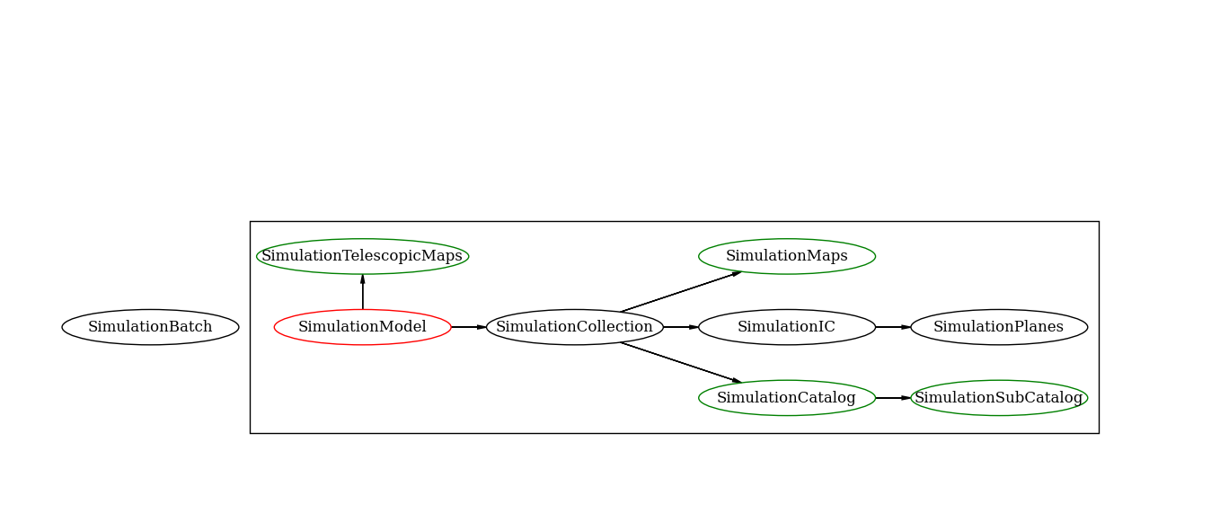
Class inheritance
This is a simplifying scheme of the class inheritance used in the lenstools pipeline